Individual Report

Author

Evelyn Rodriguez

Introduction

New York City’s 311 service fields 3-4 million requests each year from all five boroughs that cover a range of issues handled by the city’s numerous agencies. In recent years, the slow resolution times of certain responding agencies has come under fire leading to a closer examination of what could possibly take these issues so long to resolve. While much high level work has been done around the basic statistical makeup of 311 service requests, what has been missing is a deeper look into the contributing factors of long resolution times.

As part of a larger analysis into what factors drive 311 service request response and resolution times, I will explore the question How do weather conditions impact response time across agencies? My meteorological research angle is unique from the other factors explored in the main report because it is a truly unpredictable factor outside of human control quite unlike agency administration or resident income level.

Using 311 service request data from NYC OpenData and historical weather data from Open-Meteo from 2022-2025, I will analyze if and how adverse weather such as high precipitation, snow, or extreme heat/cold can affect the composition of complaints lodged and how fast agencies respond to service requests. I will further drill in at the borough level to see if there are any significant differences in response time across boroughs to take into account that different borough geographies may experience adverse weather differently.

Data Sources

NYC OpenData: 311 Service Requests from 2020 to Present

  • Main repository of inbound 311 Service Requests with key request details: creation/closure date, issue type and details, responding agency, latitude/longitude coordinates.

Open-Meteo

  • Historical weather API with data from National Weather Service with various measures of precipitation and temperature.

Data Acquisition & Preparation

Display Code
## Read the pre-processed parquet files produced by fetch_data.R

# Weather data: 23,376 rows (16 points across 5 boroughs x 1,461 days)
weather <- read_parquet("data/individual/weather/weather_clean.parquet")

# Clean 311 data: ~13M rows, may take a moment to load
nyc_311 <- read_parquet("data/individual/nyc_311_clean.parquet")

# Joined dataset: 311 requests with weather data
nyc_311_with_weather <- read_parquet("data/individual/nyc_311_with_weather.parquet")

Data Acquisition

There were three main steps for data acquisition: acquire 311 Service Request data set from NYC OpenData, acquire weather data from Open-Meteo, and finally join the two sets together spatially by latitude and longitude coordinates.

I created a separate script fetch_data.R that is run once manually to download and cache all data into parquet files. I chose parquet over CSV because CSV would process slowly and be memory-inefficient as it offers no compression. Parquet, a binary file format, is a better choice for this particular project due to the large volume of data (~13M rows). Parquet’s compression makes file sizes significantly smaller and also preserves data types directly provided by the source API, so the data downloads faster and uses significantly less memory.

311 Data

I utilized NYC OpenData’s Socrata API to pull in and cache the 311 data. This API caps each call at 50,000 rows per page so the initial fetch takes around an hour. I pull 311 service records that had an opened date between 2022-2025 and whose status was ‘Closed’ for a clear calculation for resolution time (Date Created - Date Closed).

Historical Weather Data

I gathered daily weather information for 16 weather points across NYC from 2022 to 2025 in American units (F, in). I assigned 3 weather points per borough (Brooklyn South, Brooklyn North, Brooklyn Center, etc) with the exception of Queens, which has 4 weather points in order to account for boundaries that reach down to Rockaway Beach. The intent is to account for any meteorological differences related to geography. For each day and location, I pulled daily minimum temperature, maximum temperature, total precipitation, total snowfall and max wind speed.

Using this preliminary data and guidelines from the National Weather Service for extreme cold, extreme heat, and high precipitation/snow, each day for each location was classified into three weather categories: Normal (no adverse weather occurred), Adverse (one adverse weather condition was recorded), Extreme (two or more adverse weather conditions were recorded). I also assigned a dominant weather condition so that we could discern between snow days, rainy days or hot/cold days.

Joining Both Data Sets

Once both data sets were downloaded and saved, I joined 311 records that contained both longitude/latitude coordinates and a designated borough with the weather data set to assign a weather category to each record based on creation date. Using a nearest-neighbor approach, I mapped over each 311 record and matched it to the closest weather coordinate within its borough using the coordinates in the record. This resulted in a unified data frame that contained all relevant 311 service requests with weather information.

Snapshot and Limitations of Data Acquired

NoteAcquired Data Snapshot
  • 13,195,984 service request records acquired from NYC OpenData and 23,376 from Open-Meteo
    • 193,283 (1.46%) 311 records lacked geographic coordinates and could not be matched to a weather point.
  • The 311 data set spans 2022-01-01 to 2025-12-31.
ImportantLimitations in Analysis

Data Limitations

  • Open-Meteo uses ERA5 reanalysis model rather than direct station readings so it uses modeled estimates rather than observed measurements.

Methodological Limitations

  • Resolution time is used as a proxy for service quality so a closed request does not necessarily mean the issue was resolved satisfactorily.

  • Sub-1-minute closures (316,472 records / 2.4%) likely represent automated or duplicate closures rather than genuine resolutions and their inclusion may affect agency-level averages

  • temp_min_f (daily minimum temperature) used for cold weather classification instead of daily average minimums in order to capture overnight lows which may drive infrastructure stress (ex: freezing pipes) but may not reflect daytime conditions experienced by residents

Scope Limitations

  • Four year window (2022-2025) may not capture longer-term seasonal patterns or anomalous weather years

  • 16 borough-level weather coordinate points are the finest geographic unit for weather matching. There is potential for more granular calculations in the future with more points to capture community districts or neighborhoods.

EDA: NYC 311 Requests & Weather in NYC

Weather Patterns in NYC (2022–2025)

Adverse and Extreme Weather Days by Borough

Display Code
# Count of days per weather category per borough
# Aggregated to borough level using the most common weather category
# across all points within the borough on each day
weather_category_by_borough <- weather |>
  group_by(borough, date) |>
  summarise(
    # Most common category across all points in the borough that day
    weather_category = names(which.max(table(weather_category))),
    .groups = "drop"
  ) |>
  mutate(
    weather_category = factor(weather_category,
                              levels = c("Normal", "Adverse", "Extreme"),
                              ordered = TRUE)
  ) |>
  count(borough, weather_category)

# Stacked bar chart: count of Normal/Adverse/Extreme days by borough
weather_conditions_by_borough <- ggplot(weather_category_by_borough,
       aes(x = borough, y = n, fill = weather_category)) +
  geom_col(width = 0.6) +
  # Labels for Normal and Adverse — centered inside their segments
  geom_text(
    data     = weather_category_by_borough |> 
                 filter(weather_category != "Extreme"),
    aes(label = comma(n)),
    position = position_stack(vjust = 0.5),
    size     = 3,
    color    = "white",
    fontface = "bold"
  ) +
  # Label for Extreme — positioned above the full bar
  geom_text(
    data     = weather_category_by_borough |> 
                 filter(weather_category == "Extreme"),
    aes(label = paste0("Extreme: ", comma(n)),
        y     = 0),
    vjust    = 1.0,
    size     = 2.5,
    color    = "#e74c3c",
    fontface = "bold"
  ) +
  scale_fill_manual(
    values = c(Normal  = "#2ecc71",
               Adverse = "#f39c12",
               Extreme = "#e74c3c"),
    name = "Weather Category"
  ) +
  scale_y_continuous(labels = comma) +
  labs(
    title    = "Weather Conditions by Borough (2022-2025)",
    subtitle = "Number of days classified as Normal, Adverse, or Extreme",
    x        = NULL,
    y        = "Number of Days"
  ) +
  theme_bw() +
  theme(
    legend.position = "bottom",
    plot.title      = element_text(face = "bold"),
    plot.subtitle   = element_text(color = "gray40")
  )

weather_conditions_by_borough

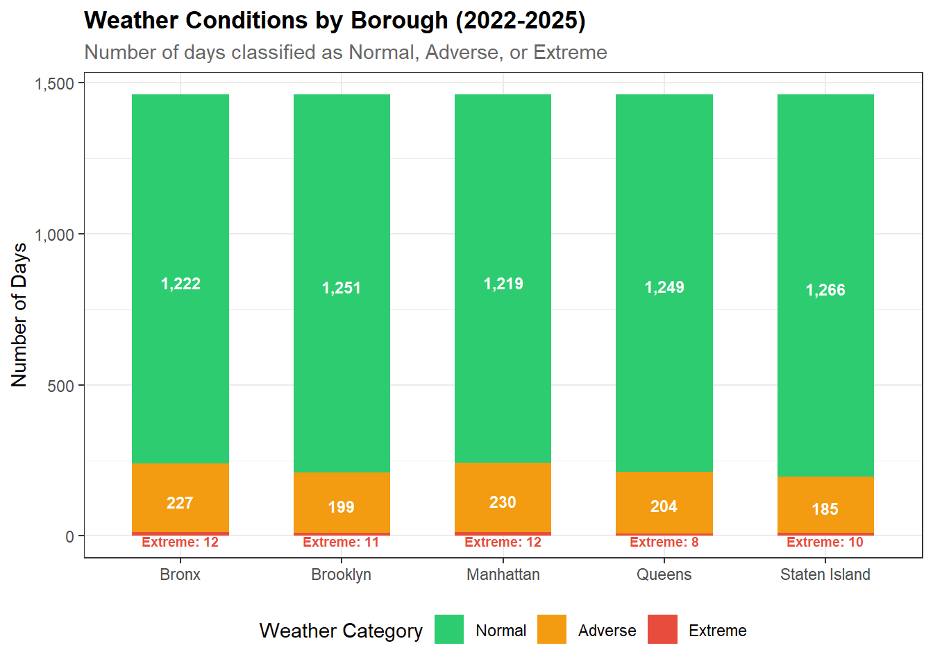
Normal weather days dominate across all 5 boroughs as expected. The Bronx and Manhattan experienced the most Adverse days and Staten Island experienced the fewest. Extreme days are rare.

Weather Event Calendar

Hover over calendar for more detailed borough weather information by month and year.

Display Code
# Heatmap: weather category by day of year, faceted by year
# Shows seasonality of adverse/extreme weather events

# Aggregate daily weather categories to monthly proportions per borough
# For each borough-month combination, calculate the proportion of days
# that were classified as Adverse or Extreme
weather_heatmap <- weather |>
  # Step 1: get one category per borough per day using most common method
  group_by(borough, date) |>
  summarise(
    weather_category = names(which.max(table(weather_category))),
    .groups = "drop"
  ) |>
  # Step 2: aggregate to monthly proportions per borough
  mutate(month = floor_date(date, "month")) |>
  group_by(borough, month) |>
  summarise(
    n_days          = n(),
    n_adverse       = sum(weather_category == "Adverse"),
    n_extreme       = sum(weather_category == "Extreme"),
    pct_adverse     = mean(weather_category %in% c("Adverse", "Extreme")) * 100,
    .groups         = "drop"
  )

# Monthly heatmap: proportion of adverse/extreme days by borough
weather_adverse_heatmap <- ggplot(weather_heatmap,
       aes(x = month, y = borough, fill = pct_adverse,
           text = paste0(
             "Borough: ", borough, "\n",
             "Month: ", format(month, "%B %Y"), "\n",
             "Adverse Days: ", n_adverse, "\n",
             "Extreme Days: ", n_extreme, "\n",
             "Total Days: ", n_days, "\n",
             "% Adverse/Extreme: ", round(pct_adverse, 1), "%"
           ))) +
  geom_tile(color = "white", linewidth = 0.3) +
  scale_fill_gradient(
    low  = "#ffffff",
    high = "#e74c3c",
    name = "% Adverse/\nExtreme Days"
  ) +
  scale_x_date(
    date_breaks = "3 months",
    date_labels = "%b %Y"
  ) +
  labs(
    title    = "Monthly Adverse & Extreme Weather Days by Borough (2022-2025)",
    subtitle = "Percentage of days per month classified as Adverse or Extreme",
    x        = NULL,
    y        = NULL,
    caption = "Source: NYC Open Data — 311 Service Requests (2022-2025)"
  ) +
  theme_bw() +
  theme(
    plot.title      = element_text(face = "bold"),
    plot.subtitle   = element_text(color = "gray40"),
    axis.text.x     = element_text(angle = 45, hjust = 1),
    legend.position = "right"
  )

# Convert to interactive plotly chart with custom tooltip
ggplotly(weather_adverse_heatmap, tooltip = "text")
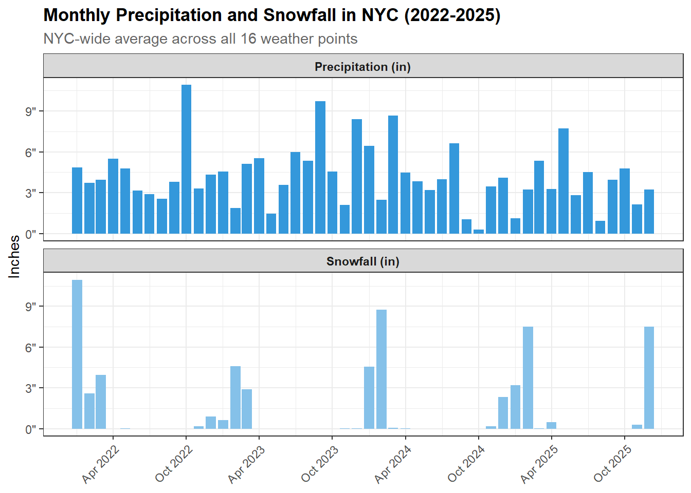
  • Winter months (Jan/Feb) show the darkest reds across all boroughs indicating high proportion of adverse/extreme days driven by cold temperatures

    • January 2022 in the Bronx shows 77% adverse/extreme days making it the coldest January (Winter Storm Kenan)
  • Summer months show lighter colors with some mid-range reds in July/August indicating heat events

    • July and August 2022 have highest percentage of adverse days likely due to heat events (32%)
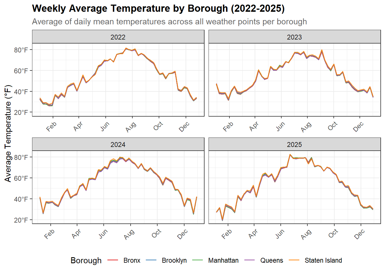
  • Patterns are consistent across boroughs which reinforces our earlier finding that weather conditions don’t vary dramatically between boroughs

311 Service Request Overview

Request Volume

Display Code
# Bar chart: total requests by borough and year
# Use plotly for interactivity

# Count of 311 requests by year
requests_by_year <- nyc_311 |>
  mutate(year = year(date)) |>
  count(year)

# Line chart: total 311 service requests by year
requests_by_year_chart <- ggplot(requests_by_year,
       aes(x = year, y = n)) +
  geom_line(color = "#3498db", linewidth = 1) +
  geom_point(color = "#3498db", size = 3) +
  geom_text(
    aes(label = comma(n),
            hjust = ifelse(year == 2022, -0.1, 0.5)),
    vjust    = -1,
    size     = 3.5,
    fontface = "bold"
  ) +
  scale_x_continuous(breaks = c(2022, 2023, 2024, 2025)) +
  scale_y_continuous(
    labels = comma,
    expand = expansion(mult = c(0.05, 0.1))
  ) +
  labs(
    title    = "NYC 311 Service Requests by Year (2022-2025)",
    subtitle = "Total closed service requests per year",
    x        = NULL,
    y        = "Number of Requests",
    caption = "Source: NYC Open Data — 311 Service Requests (2022-2025)"
  ) +
  theme_bw() +
  theme(
    plot.title    = element_text(face = "bold"),
    plot.subtitle = element_text(color = "gray40")
  )

requests_by_year_borough <- nyc_311 |>
  mutate(year = year(date)) |>
  count(year, borough) |>
  filter(!is.na(borough))


# Net growth of 311 requests by borough from 2022 to 2025
requests_growth <- requests_by_year_borough |>
  filter(year %in% c(2022, 2025)) |>
  pivot_wider(names_from = year, values_from = n, names_prefix = "year_") |>
  mutate(
    net_growth     = year_2025 - year_2022,
    pct_growth     = round((year_2025 - year_2022) / year_2022 * 100, 1)
  ) |>
  arrange(desc(pct_growth))

# Horizontal bar chart: net growth of 311 requests by borough (2022-2025)
requests_growth_chart <- ggplot(requests_growth,
       aes(x = pct_growth, y = reorder(borough, pct_growth))) +
  geom_col(fill = "#3498db", width = 0.6) +
  geom_text(
    aes(label = paste0(pct_growth, "%")),
    hjust    = -0.2,
    size     = 3.5,
    fontface = "bold"
  ) +
  scale_x_continuous(
    labels = \(x) paste0(x, "%"),
    expand = expansion(mult = c(0, 0.15))
  ) +
  labs(
    title    = "Net Growth in 311 Service Requests by Borough (2022-2025)",
    subtitle = "Percentage increase in closed service requests from 2022 to 2025",
    x        = "Percentage Growth",
    y        = NULL,
    caption = "Source: NYC Open Data — 311 Service Requests (2022-2025)"
  ) +
  theme_bw() +
  theme(
    plot.title    = element_text(face = "bold"),
    plot.subtitle = element_text(color = "gray40")
  )

requests_by_year_chart

Display Code
requests_growth_chart

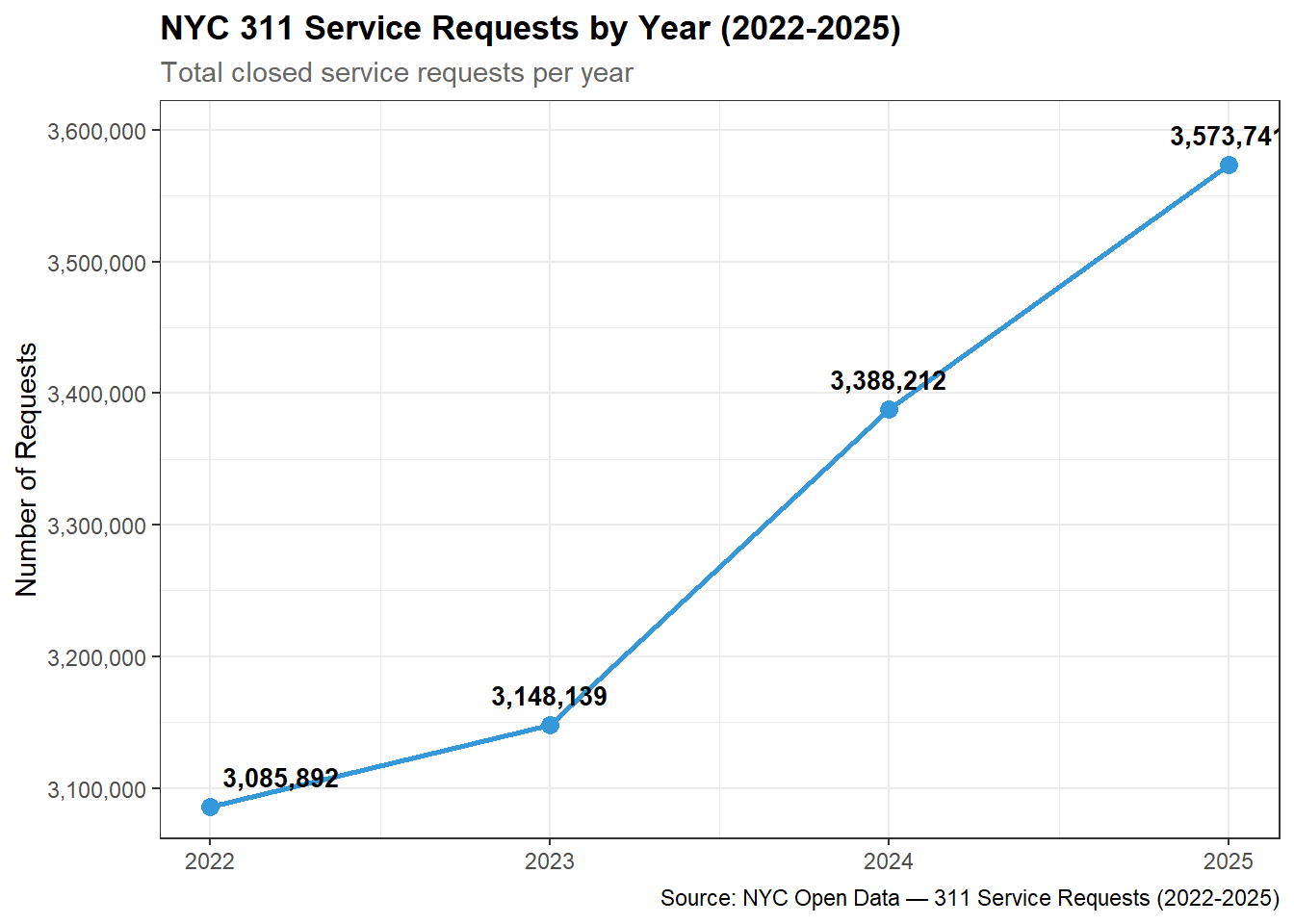
  • The number of service requests has steadily increased over time with 2025 receiving over 500,000 more requests than 2022.

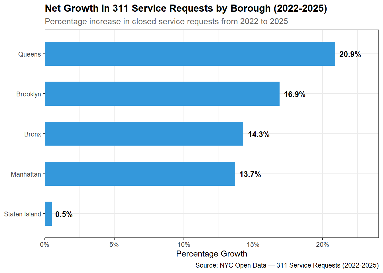
  • Queens shows the strongest and most consistent growth of any borough from 703,600 requests in 2022 to 850,735 in 2025, a 21% increase over the period. This suggests Queens residents are increasingly engaging with 311.

  • Staten Island has the lowest engagement with 311 with relatively flat growth across all four years

Top Complaint Types and Agencies

Top Complaints

Display Code
# Horizontal bar chart: top 20 complaint types
# Highlight weather-sensitive types in a different color

# Normalize complaint types to uppercase to catch all casing duplicates
# then aggregate counts and find top 2 agencies for each type
top_complaint_types <- nyc_311 |>
  mutate(complaint_type = str_to_upper(str_trim(complaint_type))) |>
  count(complaint_type, sort = TRUE) |>
  slice_head(n = 15)

# For each of the top 15 complaint types, find the top 2 responding agencies
top_complaint_agencies <- nyc_311 |>
  mutate(complaint_type = str_to_upper(str_trim(complaint_type))) |>
  filter(complaint_type %in% top_complaint_types$complaint_type) |>
  count(complaint_type, agency, sort = TRUE) |>
  group_by(complaint_type) |>
  slice_head(n = 2) |>
  summarise(
    top_agencies = paste(agency, collapse = "/"),
    .groups = "drop"
  )

# Join complaint counts with top agency labels
top_complaints_with_agencies <- top_complaint_types |>
  left_join(top_complaint_agencies, by = "complaint_type")

# Extract primary agency for color fill
top_complaints_with_agencies <- top_complaints_with_agencies |>
  mutate(
    primary_agency = str_extract(top_agencies, "^[^/]+"),
    # Reorder by count for horizontal bar chart
    complaint_type = fct_reorder(complaint_type, n)
  )

# Define color palette for agencies
agency_colors <- c(
  "NYPD" = "#2980b9",
  "HPD"  = "#e74c3c",
  "DOT"  = "#27ae60",
  "DEP"  = "#8e44ad",
  "DSNY" = "#f39c12",
  "DOB"  = "#16a085"
)

# Horizontal bar chart: top 15 complaint types colored by primary agency
# with top 2 agencies labeled on each bar
top_complaints_chart <- ggplot(top_complaints_with_agencies,
       aes(x = n, y = complaint_type, fill = primary_agency)) +
  geom_col(width = 0.7) +
  geom_text(
    aes(label = paste0(top_agencies, "  ")),
    hjust    = 1,
    size     = 3,
    color    = "white",
    fontface = "bold"
  ) +
  scale_fill_manual(values = agency_colors, name = "Primary Agency") +
  scale_x_continuous(labels = comma) +
  labs(
    title    = "Top 15 NYC 311 Complaint Types (2022-2025)",
    subtitle = "And their primary responding agency",
    x        = "Number of Requests",
    y        = NULL,
    caption = "Source: NYC Open Data — 311 Service Requests (2022-2025)"
  ) +
  theme_bw() +
  theme(
    plot.title      = element_text(face = "bold"),
    plot.subtitle   = element_text(color = "gray40"),
    legend.position = "bottom"
  )

top_complaints_chart

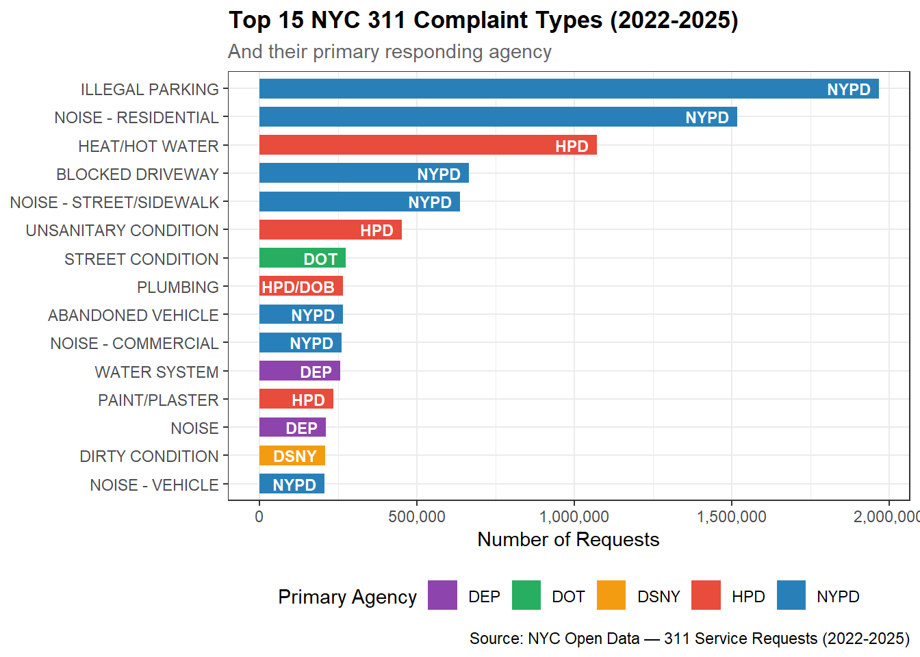
Illegal Parking, Noise (Residential), and Heat/Hot Water were the top three complaints from 2022-2025. Out of the top 5 complaints, NYPD was a primary responder for 4 of them, while HPD handles Heat/Hot Water.

Top Responding Agencies

Display Code
# Bar chart: top 10 agencies by request volume

# Count of 311 requests by agency, normalized to uppercase to catch
# any casing inconsistencies, top 10 by volume
n_total_requests <- nrow(nyc_311)

top_agencies <- nyc_311 |>
  mutate(agency_name = str_to_upper(str_trim(agency_name))) |>
  count(agency_name, sort = TRUE) |>
  slice_head(n = 10) |>
  mutate(
    # Percentage of all 13.2M requests handled by each agency
    pct_total   = round(n / n_total_requests * 100, 1),
    agency_name = fct_reorder(agency_name, n)
  )

# GT table: top 10 responding agencies by request volume
top_agencies_table <- top_agencies |>
  arrange(desc(n)) |>
  select(agency_name, n, pct_total) |>
  mutate(
    # Convert agency names from uppercase to title case for readability
    agency_name = str_to_title(str_to_lower(agency_name))
  ) |>
  gt() |>
  tab_header(
    title    = "Top 10 Responding Agencies by 311 Request Volume (2022-2025)",
    subtitle = "Total closed service requests per agency"
  ) |>
  cols_label(
    agency_name = "Agency",
    n           = "Requests",
    pct_total   = "% of Total"
  ) |>
  fmt_number(columns = n, decimals = 0) |>
  fmt_number(columns = pct_total, decimals = 1, suffix = "%") |>
  cols_align(align = "left",  columns = agency_name) |>
  cols_align(align = "right", columns = c(n, pct_total)) |>
  tab_style(
    style     = cell_text(weight = "bold"),
    locations = cells_column_labels()
  ) |>
  tab_style(
    style     = cell_fill(color = "#f2f2f2"),
    locations = cells_body(rows = seq(1, 10, by = 2))
  ) |>
  tab_source_note(
    source_note = "Source: NYC Open Data — 311 Service Requests (2022-2025)"
  )

top_agencies_table
Top 10 Responding Agencies by 311 Request Volume (2022-2025)
Total closed service requests per agency
Agency Requests % of Total
New York City Police Department 6,040,445 45.8
Department Of Housing Preservation And Development 2,841,133 21.5
Department Of Sanitation 1,229,080 9.3
Department Of Transportation 818,500 6.2
Department Of Environmental Protection 719,679 5.5
Department Of Parks And Recreation 407,798 3.1
Department Of Buildings 386,921 2.9
Department Of Health And Mental Hygiene 314,027 2.4
Department Of Homeless Services 142,713 1.1
Taxi And Limousine Commission 121,113 0.9
Source: NYC Open Data — 311 Service Requests (2022-2025)

Judging by the number of closed service requests, NYPD is the #1 responding agency closing over 6M requests (46%). Given that 4 of the top 5 311 complaints are handled primarily by NYPD, this is line with expectations. Combined with HPD, the second largest closer, both agencies closed a combined total of 68% of all service requests.

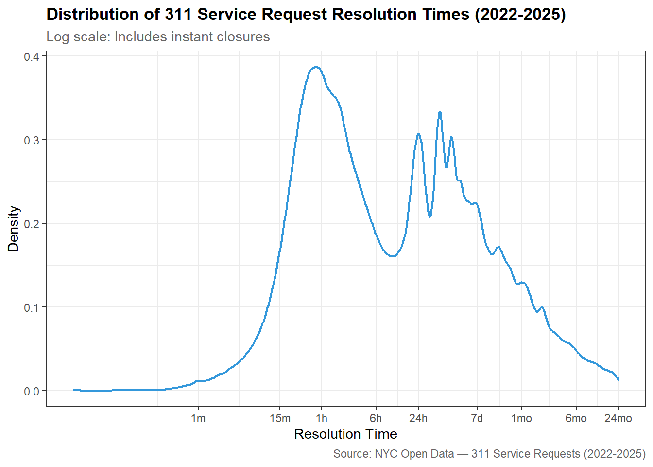
Resolution Time Distribution

Resolution Time Categories

  • Instant: < 0.017 hrs (under 1 minute)
  • Fast: 0.017 to 1 hr
  • Standard: 1 to 24 hrs
  • Extended: 24 to 720 hrs (1 month)
  • Long-term: over 720 hrs
Display Code
# Histogram or density plot of resolution times (log scale)
# Annotate the median and key percentiles

# Resolution time distribution data
# Version 1: all records excluding exact zeros (log scale requires > 0)
resolution_dist_all <- nyc_311 |>
  filter(resolution_hrs > 0) |>
  select(resolution_hrs)

# Resolution time categories
# Applied to full dataset including instant closures
resolution_categories <- nyc_311 |>
  mutate(
    resolution_category = case_when(
      resolution_hrs <  0.017             ~ "Instant",
      resolution_hrs <  1                 ~ "Fast",
      resolution_hrs <  24                ~ "Standard",
      resolution_hrs <  720               ~ "Extended",
      TRUE                                ~ "Long-term"
    ) |> factor(levels = c("Instant", "Fast", "Standard",
                            "Extended", "Long-term"),
                ordered = TRUE)
  ) |>
  count(resolution_category) |>
  mutate(pct = round(n / sum(n) * 100, 1))


# Density plot: resolution time distribution on log scale
resolution_density <- ggplot(resolution_dist_all,
       aes(x = resolution_hrs)) +
  geom_density(
    color     = "#3498db",
    linewidth = 0.8
  ) +
  scale_x_log10(
    labels = \(x) case_when(
      x < 1    ~ paste0(round(x * 60), "m"),
      x < 24   ~ paste0(round(x), "h"),
      x < 720  ~ paste0(round(x / 24), "d"),
      TRUE     ~ paste0(round(x / 720), "mo")
    ),
    breaks = c(0.017, 0.25, 1, 6, 24, 168, 720, 4380, 17520)
  ) +
  labs(
    title   = "Distribution of 311 Service Request Resolution Times (2022-2025)",
    subtitle = "Log scale: Includes instant closures",
    x       = "Resolution Time",
    y       = "Density",
    caption = "Source: NYC Open Data — 311 Service Requests (2022-2025)"
  ) +
  theme_bw() +
  theme(
    plot.title    = element_text(face = "bold"),
    plot.subtitle = element_text(color = "gray40"),
    plot.caption  = element_text(color = "gray40")
  )

# GT table: percentage of requests by resolution time category
resolution_categories_table <- resolution_categories |>
  mutate(resolution_category = as.character(resolution_category)) |>
  gt() |>
  tab_header(
    title    = "311 Service Requests by Resolution Time Category (2022-2025)",
    subtitle = "Distribution of closed service requests across resolution time categories"
  ) |>
  cols_label(
    resolution_category = "Resolution Category",
    n                   = "Requests",
    pct                 = "% of Total"
  ) |>
  fmt_number(columns = n,   decimals = 0) |>
  fmt_number(columns = pct, decimals = 1, suffix = "%") |>
  cols_align(align = "left",  columns = resolution_category) |>
  cols_align(align = "right", columns = c(n, pct)) |>
  tab_style(
    style     = cell_text(weight = "bold"),
    locations = cells_column_labels()
  ) |>
  tab_style(
    style     = cell_fill(color = "#f2f2f2"),
    locations = cells_body(rows = seq(1, 5, by = 2))
  ) |>
  tab_source_note(
    source_note = "Source: NYC Open Data — 311 Service Requests (2022-2025)"
  )

resolution_density

Display Code
resolution_categories_table
311 Service Requests by Resolution Time Category (2022-2025)
Distribution of closed service requests across resolution time categories
Resolution Category Requests % of Total
Instant 316,472 2.4
Fast 3,204,422 24.3
Standard 4,420,194 33.5
Extended 4,168,833 31.6
Long-term 1,086,063 8.2
Source: NYC Open Data — 311 Service Requests (2022-2025)

Nearly a quarter of all requests were resolved within an hour. 58% of service requests were closed within the Fast + Standard resolution times (within 24 hours).

Two peaks appear in the resolution time distribution: one around 1 hour and another around 24-48 hours. A long tail shows that 8.2% of requests extend to months. This bimodal pattern suggests two distinct types of resolution behavior in the data.

ImportantMean vs Median

Due to the heavy skew, the mean is much larger than the median so we will rely on median for a more reliable measure.

Seasonal Patterns

Display Code
# Line chart: monthly request volume over 2022-2025
# Facet or color by complaint type category

# Identify the 28 complaint types that account for 80% of all requests
top_complaint_types_80 <- nyc_311 |>
  mutate(complaint_type = str_to_upper(str_trim(complaint_type))) |>
  count(complaint_type, sort = TRUE) |>
  mutate(
    pct            = n / sum(n) * 100,
    cumulative_pct = cumsum(pct)
  ) |>
  filter(cumulative_pct <= 80) |>
  pull(complaint_type)

# Compute average monthly request volume per complaint type
# averaged across all 4 years
seasonal_patterns <- nyc_311 |>
  mutate(
    complaint_type = str_to_upper(str_trim(complaint_type)),
    month_num      = month(date),
    month_name     = month(date, label = TRUE, abbr = TRUE)
  ) |>
  filter(complaint_type %in% top_complaint_types_80) |>
  count(complaint_type, month_num, month_name) |>
  # Divide by 4 to get average monthly volume across the 4 year period
  mutate(avg_monthly = n / 4)

# Heatmap: average monthly request volume by complaint type (2022-2025)
# Rows = complaint types, columns = months, color = avg monthly volume
seasonal_heatmap <- ggplot(seasonal_patterns,
       aes(x = month_name, 
           y = reorder(complaint_type, avg_monthly),
           fill = avg_monthly)) +
  geom_tile(color = "white", linewidth = 0.3) +
  scale_fill_gradient(
    low    = "#ffffff",
    high   = "#2980b9",
    limits = c(0, 40000),
    oob    = scales::squish,
    name   = "Avg Monthly\nRequests\n(capped at 30k)"
  ) +
  scale_x_discrete(position = "top") +
  labs(
    title   = "Seasonal Patterns in NYC 311 Requests by Complaint Type",
    subtitle = "Average monthly request volume across 2022-2025",
    x        = NULL,
    y        = NULL,
    caption  = "Source: NYC Open Dat: 311 Service Requests (2022-2025)"
  ) +
  theme_bw() +
  theme(
    plot.title    = element_text(face = "bold", size = 12),
    plot.subtitle = element_text(color = "gray40"),
    plot.caption  = element_text(color = "gray40"),
    axis.text.y   = element_text(size = 8),
    legend.position = "right"
  )

seasonal_heatmap

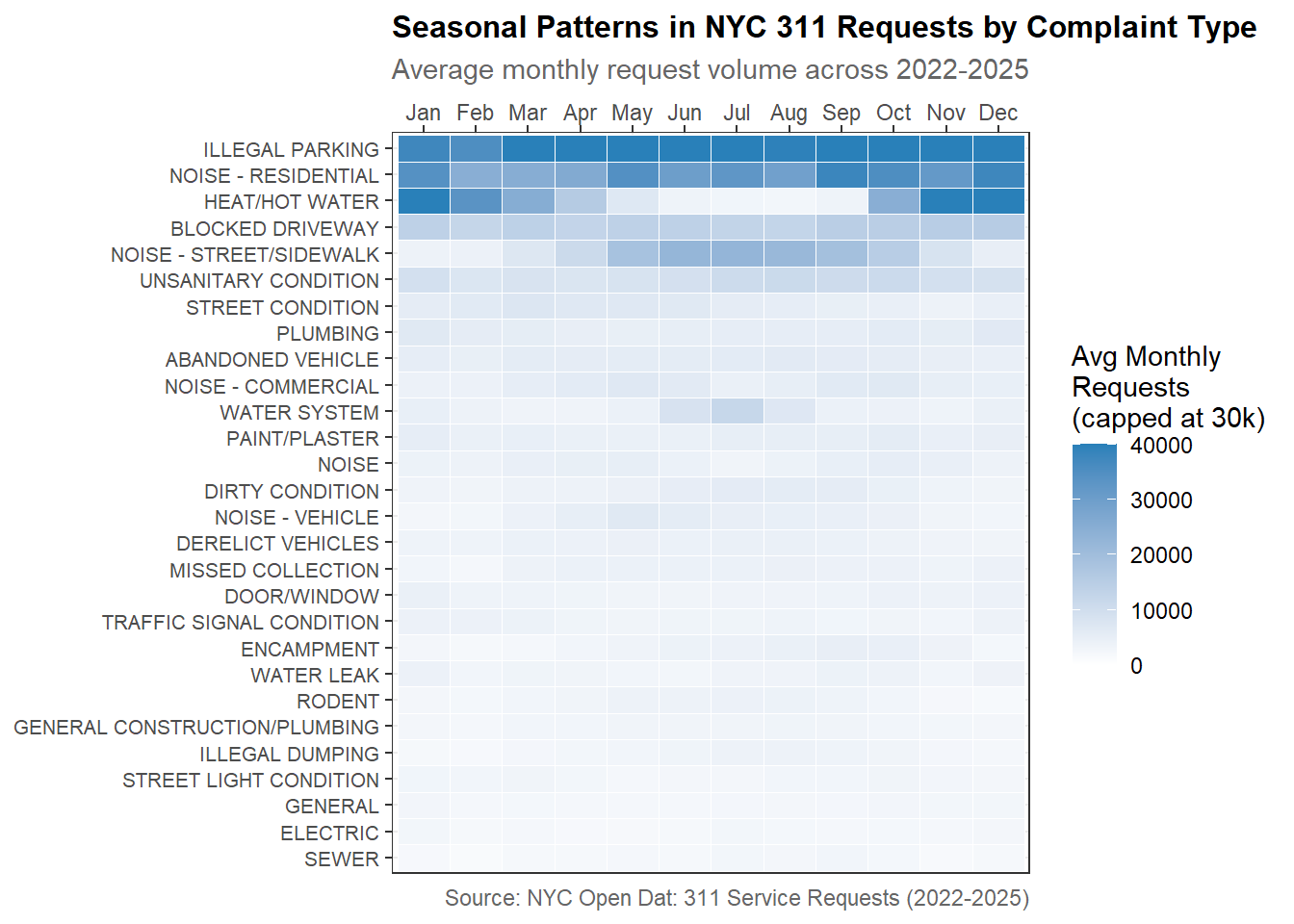
Among the top complaints, some clear seasonal patterns emerge:

  • Heat/Hot Water: darkest in winter months (Jan-Mar, Nov-Dec) and nearly white in summer indicating these complaints are driven by the colder season.

  • Noise (Residential & Street/Sidewalk): slightly darker in summer months

  • Illegal Parking: consistently high year-round unlike most complaint types that show clear seasonal peaks

Weather × Resolution Time Analysis

Resolution Times by Weather Category

Display Code
# Box plot or violin plot: resolution time distribution by weather category
# Use log scale on y-axis given the skewed distribution

# Working data set for Section 6 analysis
# Excludes 196,803 records with missing weather data
nyc_311_weather_analysis <- nyc_311_with_weather |>
  filter(!is.na(weather_category))

# Median resolution times by weather category
# Using median rather than mean due to heavy right skew in resolution times
resolution_by_weather <- nyc_311_weather_analysis |>
  group_by(weather_category) |>
  summarise(
    n_requests  = n(),
    median_hrs  = median(resolution_hrs, na.rm = TRUE),
    mean_hrs    = mean(resolution_hrs,   na.rm = TRUE),
    p25_hrs     = quantile(resolution_hrs, 0.25, na.rm = TRUE),
    p75_hrs     = quantile(resolution_hrs, 0.75, na.rm = TRUE),
    .groups     = "drop"
  )

# Bar chart: median resolution time by weather category
resolution_by_weather_chart <- ggplot(resolution_by_weather,
       aes(x = weather_category, y = median_hrs, fill = weather_category)) +
  geom_col(width = 0.6) +
  # IQR shown as error bars (p25 to p75)
  geom_errorbar(
    aes(ymin = p25_hrs, ymax = p75_hrs),
    width     = 0.2,
    linewidth = 0.8,
    color     = "gray30"
  ) +  
  geom_text(
    aes(label = paste0(round(median_hrs, 1), " hrs")),
    vjust    = -0.5,
    size     = 3.5,
    fontface = "bold"
  ) +
  scale_fill_manual(
    values = c(Normal  = "#2ecc71",
               Adverse = "#f39c12",
               Extreme = "#e74c3c"),
    name = "Weather Category"
  ) +
  scale_y_continuous(
    labels = \(x) paste0(x, " hrs"),
    expand = expansion(mult = c(0, 0.1))
  ) +
  labs(
    title    = "Median 311 Resolution Time by Weather Category (2022-2025)",
    subtitle = "Across All Complaint Types",
    x        = NULL,
    y        = "Median Resolution Time (hrs)",
    caption  = "Sources: NYC Open Data — 311 Service Requests; Open-Meteo Historical Archive API (2022-2025)"
  ) +
  theme_bw() +
  theme(
    plot.title      = element_text(face = "bold"),
    plot.subtitle   = element_text(color = "gray40"),
    plot.caption    = element_text(color = "gray40"),
    legend.position = "none"
  )

resolution_by_weather_chart

Display Code
# Median resolution times by dominant weather condition
# Excludes "Clear" since that corresponds to Normal weather days
resolution_by_condition <- nyc_311_weather_analysis |>
  filter(dominant_condition != "Clear") |>
  group_by(dominant_condition, weather_category) |>
  summarise(
    n_requests = n(),
    median_hrs = median(resolution_hrs, na.rm = TRUE),
    p25_hrs    = quantile(resolution_hrs, 0.25, na.rm = TRUE),
    p75_hrs    = quantile(resolution_hrs, 0.75, na.rm = TRUE),
    .groups    = "drop"
  )

# Bar chart: median resolution time by dominant weather condition
# with reference line showing Normal day median for comparison
resolution_by_condition_chart <- ggplot(resolution_by_condition,
       aes(x = reorder(dominant_condition, median_hrs),
           y = median_hrs,
           fill = weather_category)) +
  geom_col(position = "dodge", width = 0.6) +
  # Reference line showing Normal day median for comparison
  geom_hline(
    yintercept = 6.02,
    color      = "#2ecc71",
    linewidth  = 0.8,
    linetype   = "dashed"
  ) +
  # Label for reference line
  annotate(
    "text",
    x     = 0.5,
    y     = 7,
    label = "Normal: 6.02 hrs",
    color = "#2ecc71",
    size  = 3,
    hjust = 0,
    fontface = "bold"
  ) +
  geom_text(
    aes(label = paste0(round(median_hrs, 1), " hrs")),
    position = position_dodge(width = 0.6),
    vjust    = -0.5,
    size     = 3,
    fontface = "bold"
  ) +
  scale_fill_manual(
    values = c(Adverse = "#f39c12",
               Extreme = "#e74c3c"),
    name   = "Weather Category"
  ) +
  scale_y_continuous(
    labels = \(x) paste0(x, " hrs"),
    expand = expansion(mult = c(0, 0.15))
  ) +
  labs(
    title    = "Median 311 Resolution Time by Weather Condition (2022-2025)",
    subtitle = "Normal day median (dashed line) as reference",
    x        = NULL,
    y        = "Median Resolution Time (hrs)",
    caption  = "Sources: NYC Open Data — 311 Service Requests; Open-Meteo Historical Archive API (2022-2025)"
  ) +
  theme_bw() +
  theme(
    plot.title      = element_text(face = "bold"),
    plot.subtitle   = element_text(color = "gray40"),
    plot.caption    = element_text(color = "gray40"),
    legend.position = "bottom"
  )

resolution_by_condition_chart

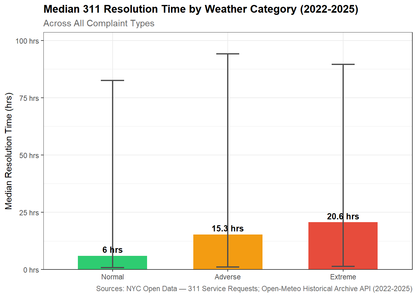
Median resolution time increases 2.5x on Adverse days (15 hours) and 3.4x on Extreme days (20 hours).

The spread of resolution times also widens meaning some requests get resolved faster while others take much longer. This suggests uneven agency responses during bad weather.

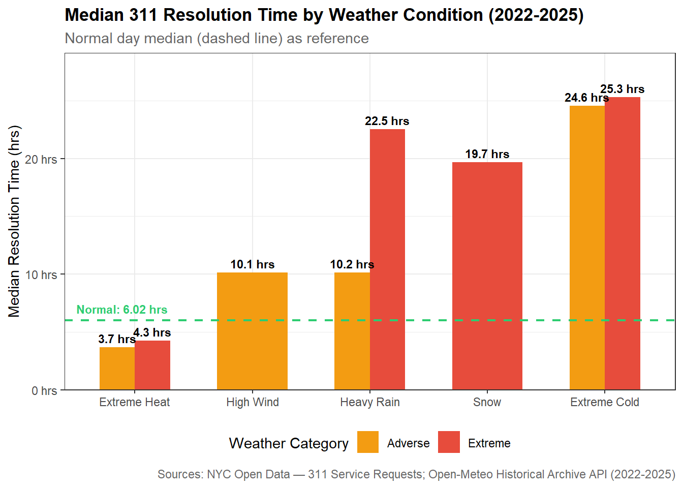
What Weather Matters Most:

  • Snow and Extreme Cold are the most disruptive.
    • Extreme Cold: longest median resolution time of any condition at nearly 25 hours (4x Normal)
    • Snow: impact is significant at 19.7 hours
  • Extreme Heat is the only condition where requests resolve faster than Normal at around 4 hours.
    • This may indicate that heat complaints get prioritized or that agencies close heat-related complaints quickly without necessarily resolving them.
  • Extreme Heavy Rain resolution is more than double Adverse Heavy Rain days. Rain compounded with other weather conditions (such as in major storms) creates a big blocker for issue resolution.

Resolution Times by Agency

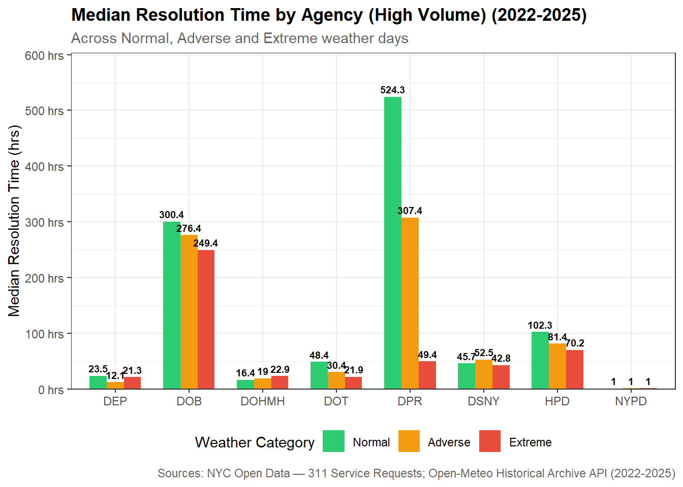
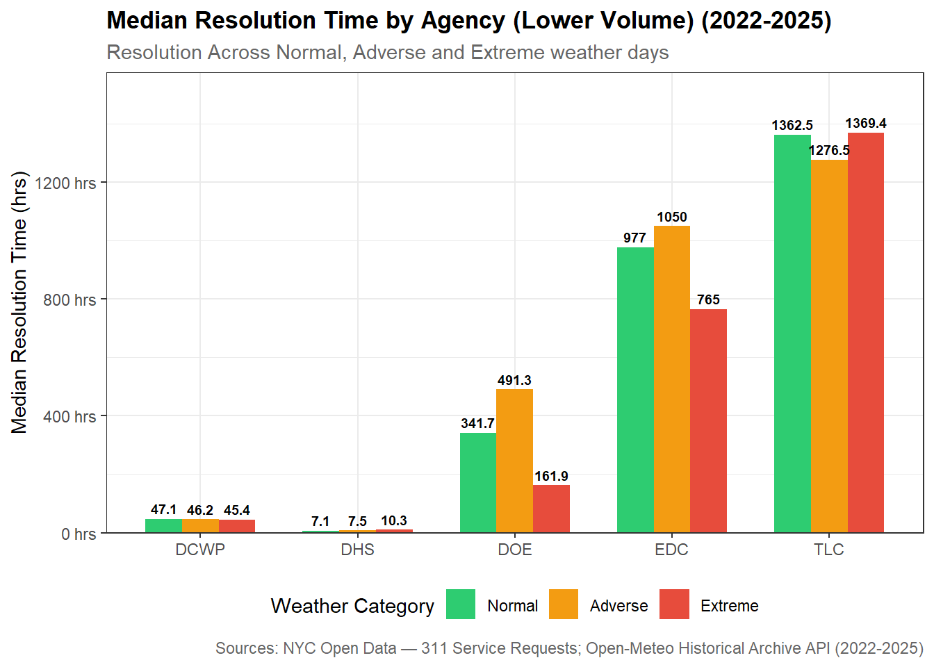
To account for major differences in request volumes between agencies, they are split up into two groups: high-volume and low-volume.

Display Code
# Median resolution time by agency and weather category - Includes all agencies
resolution_by_agency_weather <- nyc_311_weather_analysis |>
  mutate(agency = str_to_upper(str_trim(agency))) |>
  group_by(agency, weather_category) |>
  summarise(
    n_requests = n(),
    median_hrs = median(resolution_hrs, na.rm = TRUE),
    .groups    = "drop"
  )

# Free memory after heavy operation
gc()

# Split agencies into high and low volume groups
# High volume: > 100,000 requests on Normal days
# Low volume: < 100,000 requests on Normal days
# OOS and OTI excluded due to insufficient sample size
high_volume_agencies <- c("NYPD", "HPD", "DSNY", "DOT", "DEP",
                           "DPR", "DOB", "DOHMH")

low_volume_agencies  <- c("TLC", "DCWP", "DHS", "EDC", "DOE")

# Create two filtered datas ets for visualization
resolution_agency_high <- resolution_by_agency_weather |>
  filter(agency %in% high_volume_agencies)

resolution_agency_low <- resolution_by_agency_weather |>
  filter(agency %in% low_volume_agencies)

# Compute percentage change from Normal baseline for each agency
resolution_agency_pct_change <- resolution_by_agency_weather |>
  filter(agency %in% c(high_volume_agencies, low_volume_agencies)) |>
  group_by(agency) |>
  mutate(
    normal_median = median_hrs[weather_category == "Normal"],
    pct_change    = round((median_hrs - normal_median) / normal_median * 100, 1)
  ) |>
  ungroup() |>
  mutate(
    volume_group = case_when(
      agency %in% high_volume_agencies ~ "High Volume Agencies",
      agency %in% low_volume_agencies  ~ "Lower Volume Agencies"
    )
  )
Display Code
# Define a consistent color per agency across both volume groups
agency_colors <- c(
  # High volume
  "NYPD"  = "#2980b9",
  "HPD"   = "#e74c3c",
  "DSNY"  = "#f39c12",
  "DOT"   = "#27ae60",
  "DEP"   = "#8e44ad",
  "DPR"   = "#16a085",
  "DOB"   = "#d35400",
  "DOHMH" = "#c0392b",
  # Low volume
  "TLC"   = "#2c3e50",
  "DCWP"  = "#7f8c8d",
  "DHS"   = "#1abc9c",
  "EDC"   = "#e67e22",
  "DOE"   = "#9b59b6"
)

# Bar chart: median resolution time by agency and weather category
# High volume agencies
resolution_agency_high_chart <- ggplot(resolution_agency_high,
       aes(x = agency, y = median_hrs, fill = weather_category)) +
  geom_col(position = "dodge", width = 0.7) +
  geom_text(
    aes(label = round(median_hrs, 1)),
    position = position_dodge(width = 0.7),
    vjust    = -0.5,
    size     = 2.5,
    fontface = "bold"
  ) +
  scale_fill_manual(
    values = c(Normal  = "#2ecc71",
               Adverse = "#f39c12",
               Extreme = "#e74c3c"),
    name   = "Weather Category"
  ) +
  scale_y_continuous(
    labels = \(x) paste0(x, " hrs"),
    expand = expansion(mult = c(0, 0.15))
  ) +
  labs(
    title    = "Median Resolution Time by Agency (High Volume) (2022-2025)",
    subtitle = "Across Normal, Adverse and Extreme weather days",
    x        = NULL,
    y        = "Median Resolution Time (hrs)",
    caption  = "Sources: NYC Open Data — 311 Service Requests; Open-Meteo Historical Archive API (2022-2025)"
  ) +
  theme_bw() +
  theme(
    plot.title      = element_text(face = "bold"),
    plot.subtitle   = element_text(color = "gray40"),
    plot.caption    = element_text(color = "gray40"),
    legend.position = "bottom"
  )

# Bar chart: median resolution time by agency and weather category
# Low volume agencies
resolution_agency_low_chart <- ggplot(resolution_agency_low,
       aes(x = agency, y = median_hrs, fill = weather_category)) +
  geom_col(position = "dodge", width = 0.7) +
  geom_text(
    aes(label = round(median_hrs, 1)),
    position = position_dodge(width = 0.7),
    vjust    = -0.5,
    size     = 2.5,
    fontface = "bold"
  ) +
  scale_fill_manual(
    values = c(Normal  = "#2ecc71",
               Adverse = "#f39c12",
               Extreme = "#e74c3c"),
    name   = "Weather Category"
  ) +
  scale_y_continuous(
    labels = \(x) paste0(x, " hrs"),
    expand = expansion(mult = c(0, 0.15))
  ) +
  labs(
    title    = "Median Resolution Time by Agency (Lower Volume) (2022-2025)",
    subtitle = "Resolution Across Normal, Adverse and Extreme weather days",
    x        = NULL,
    y        = "Median Resolution Time (hrs)",
    caption  = "Sources: NYC Open Data — 311 Service Requests; Open-Meteo Historical Archive API (2022-2025)"
  ) +
  theme_bw() +
  theme(
    plot.title      = element_text(face = "bold"),
    plot.subtitle   = element_text(color = "gray40"),
    plot.caption    = element_text(color = "gray40"),
    legend.position = "bottom"
  )

resolution_agency_high_chart

Display Code
resolution_agency_low_chart

Display Code
# Agency x weather condition breakdown
# Separating Extreme Cold, Snow, Heat and Rain into distinct conditions
# All agencies except NYPD
resolution_agency_condition <- nyc_311_weather_analysis |>
  mutate(agency = str_to_upper(str_trim(agency))) |>
  filter(
    agency %in% c(high_volume_agencies, low_volume_agencies),
    dominant_condition %in% c("Extreme Cold", "Snow",
                               "Extreme Heat", "Heavy Rain")
  ) |>
  mutate(
    condition_group = case_when(
      dominant_condition == "Extreme Cold" ~ "Extreme Cold",
      dominant_condition == "Snow"         ~ "Snow",
      dominant_condition == "Extreme Heat" ~ "Extreme Heat",
      dominant_condition == "Heavy Rain"   ~ "Rain"
    )
  ) |>
  group_by(agency, condition_group) |>
  summarise(
    n_requests = n(),
    median_hrs = median(resolution_hrs, na.rm = TRUE),
    .groups    = "drop"
  )

# Free memory after heavy operation
gc()

# Compute overall median from full dataset per agency — must use the
# full resolution time distribution not the condition-level medians
agency_overall_median <- nyc_311_weather_analysis |>
  mutate(agency = str_to_upper(str_trim(agency))) |>
  filter(agency %in% c(high_volume_agencies, low_volume_agencies)) |>
  group_by(agency) |>
  summarise(
    overall_median = median(resolution_hrs, na.rm = TRUE),
    .groups = "drop"
  )

# Free memory after heavy operation
gc()

# Join overall median, compute percentage change and flag low sample sizes
resolution_agency_condition <- resolution_agency_condition |>
  left_join(agency_overall_median, by = "agency") |>
  mutate(
    pct_change_from_overall = round(
      (median_hrs - overall_median) / overall_median * 100, 1
    ),
    # Flag low sample size cells for grey overlay
    low_sample = n_requests < 1000
  )
Display Code
# Heatmap: % change from overall median by agency and weather condition
resolution_agency_condition_heatmap <- ggplot(resolution_agency_condition,
       aes(x = condition_group, y = agency,
           fill = ifelse(low_sample, NA, pct_change_from_overall))) +
  geom_tile(color = "white", linewidth = 0.5) +
  # Grey overlay for low sample size cells
  geom_tile(
    data  = resolution_agency_condition |> filter(low_sample),
    fill  = "gray80",
    color = "white",
    linewidth = 0.5
  ) +
  # Labels for normal cells
  geom_text(
    data     = resolution_agency_condition |> filter(!low_sample),
    aes(label = paste0(pct_change_from_overall, "%")),
    size     = 3,
    fontface = "bold",
    color    = "black"
  ) +
  # Label for low sample size cells — shows value with italic styling
  # to signal lower reliability to the reader
  geom_text(
    data     = resolution_agency_condition |> filter(low_sample),
    aes(label = paste0(pct_change_from_overall, "%*")),
    size     = 2.5,
    color    = "gray40",
    fontface = "italic"
  ) +
  scale_fill_gradient2(
    low      = "#27ae60",
    mid      = "white",
    high     = "#e74c3c",
    midpoint = 0,
    na.value = "gray80",
    name     = "% Change from\nAgency's Overall\nMedian"
  ) +
  labs(
    title    = "Weather Condition Sensitivity by Agency",
    subtitle = "% Resolution Time Change During Adverse Weather: green = faster, red = slower",
    x        = NULL,
    y        = NULL,
    caption  = "Sources: NYC Open Data — 311 Service Requests; Open-Meteo Historical Archive API (2022-2025)\n*Grey cells indicate insufficient sample size (n < 1,000)"
  ) +
  theme_bw() +
  theme(
    plot.title      = element_text(face = "bold"),
    plot.subtitle   = element_text(color = "gray40", size = 9),
    plot.caption    = element_text(color = "gray40"),
    axis.text.y     = element_text(size = 9),
    legend.position = "right"
  )

resolution_agency_condition_heatmap

Display Code
# Faceted bar chart: median resolution time by weather category
# for weather-sensitive complaint types only

# Calculate complaint volume by weather category
# then compute percentage change from Normal baseline
# to identify weather-sensitive complaint types
complaint_weather_volume <- nyc_311_weather_analysis |>
  mutate(complaint_type = str_to_upper(str_trim(complaint_type))) |>
  group_by(complaint_type, weather_category) |>
  summarise(
    n_requests = n(),
    .groups    = "drop"
  ) |>
  left_join(
    nyc_311_weather_analysis |>
      group_by(weather_category) |>
      summarise(n_days = n_distinct(date), .groups = "drop"),
    by = "weather_category"
  ) |>
  mutate(avg_daily = n_requests / n_days) |>
  group_by(complaint_type) |>
  mutate(
    # Use NA if no Normal day records exist for this complaint type
    normal_daily = ifelse(
      any(weather_category == "Normal"),
      avg_daily[weather_category == "Normal"][1],
      NA_real_
    ),
    pct_change = round((avg_daily - normal_daily) / normal_daily * 100, 1)
  ) |>
  ungroup() |>
  # Exclude complaint types with no Normal day baseline
  filter(!is.na(normal_daily))

# Show top 20 complaint types with largest spike on Adverse days
complaint_weather_volume |>
  filter(
    weather_category == "Adverse",
    normal_daily >= 10    # Exclude very low volume types
  ) |>
  arrange(desc(pct_change)) |>
  slice_head(n = 20) |>
  select(complaint_type, normal_daily, avg_daily, pct_change)

# Show top 20 complaint types with largest spike on Extreme days
complaint_weather_volume |>
  filter(
    weather_category == "Extreme",
    normal_daily >= 10
  ) |>
  arrange(desc(pct_change)) |>
  slice_head(n = 20) |>
  select(complaint_type, normal_daily, avg_daily, pct_change)


# Define weather-sensitive complaint types identified through previous steps
weather_sensitive_types <- c(
  "SNOW OR ICE",
  "HEAT/HOT WATER",
  "WATER SYSTEM",
  "DAMAGED TREE",
  "WATER LEAK"
)

# Median resolution times for weather-sensitive complaint types
# by weather category
resolution_sensitive_types <- nyc_311_weather_analysis |>
  mutate(complaint_type = str_to_upper(str_trim(complaint_type))) |>
  filter(complaint_type %in% weather_sensitive_types) |>
  group_by(complaint_type, weather_category) |>
  summarise(
    n_requests = n(),
    median_hrs = median(resolution_hrs, na.rm = TRUE),
    .groups    = "drop"
  )


# Compute percentage change from Normal baseline for each complaint type (diverging values for chart)
resolution_sensitive_pct <- resolution_sensitive_types |>
  group_by(complaint_type) |>
  mutate(
    normal_median = median_hrs[weather_category == "Normal"],
    pct_change    = round(
      (median_hrs - normal_median) / normal_median * 100, 1
    ),
    abs_change    = round(median_hrs - normal_median, 1)
  ) |>
  ungroup() |>
  filter(weather_category != "Normal")
Display Code
# Diverging bar chart: % change from Normal baseline
# Bars extend left (faster) or right (slower) from center baseline
resolution_sensitive_diverging <- ggplot(resolution_sensitive_pct,
       aes(x = pct_change,
           y = reorder(complaint_type, pct_change),
           fill = weather_category)) +
  geom_col(position = "dodge", width = 0.6) +
  geom_vline(xintercept = 0, color = "black", linewidth = 0.8) +
  geom_text(
    aes(label = paste0(ifelse(pct_change >= 0, "+", ""), pct_change, "%"),
        hjust = ifelse(pct_change >= 0, -0.1, 1.1)),
    position = position_dodge(width = 0.6),
    size     = 2.8,
    fontface = "bold"
  ) +
  scale_fill_manual(
    values = c(Adverse = "#f39c12", Extreme = "#e74c3c"),
    name   = "Weather Category"
  ) +
  scale_x_continuous(
    labels = \(x) paste0(x, "%"),
    expand = expansion(mult = c(0.2, 0.2))
  ) +
  labs(
    title    = "Weather-Sensitive Complaint Types",
    subtitle = "% Change from Normal: Left of 0% = faster resolution, Right = slower resolution",
    x        = "% Change from Normal Median",
    y        = NULL,
    caption  = "Sources: NYC Open Data — 311 Service Requests; Open-Meteo Historical Archive API (2022-2025)"
  ) +
  theme_bw() +
  theme(
    plot.title      = element_text(face = "bold"),
    plot.subtitle   = element_text(color = "gray40", size = 9),
    plot.caption    = element_text(color = "gray40"),
    legend.position = "bottom"
  )

resolution_sensitive_diverging

NoteKey Observations
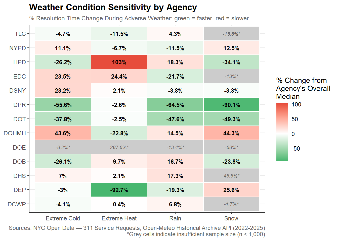
  • Field based agencies appear to be more affected by weather especially if they are responding to weather specific complaints while administrative and enforcement agencies (NYPD, DHS, DOHMH) are not as affected by bad weather.

  • While there may be some prioritization to get things closed quicker, a surge in weather specific requests may still see slower than normal resolution due to other external factors.

DOHMH showed the most consistent slowdown (-43%) for winter conditions (Extreme Cold and Snow).

HPD slows down most in extreme heat conditions usually found in Summer.

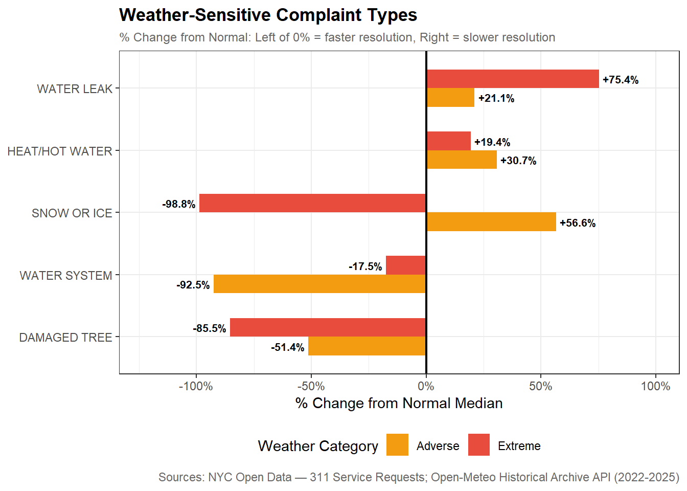
  • Requests are handled faster during Extreme Cold and Snow days (26-34% faster than normal).

  • Heat/Hot Water requests are still resolved 19-30% slower than normal.

DEP and DPR appear to have the fastest improvements on resolution time with 92% and 90% improvement respectively but further digging reveals that DEP and DPR had a high volume of instant closures for Water System complaints (DEP) and Snow/Ice complaints (DPR) during severe weather events like storms. These measures may be unreliable outliers.

  • Damaged Tree (DPR) jumps to 55% of all DPR requests vs 22% on Normal days. During Extreme weather events Damaged Tree complaints appear to flood in and get resolved quickly. This shifts the overall DPR median down dramatically. This may indicate that DPR doesn’t necessarily get faster during Extreme weather but it’s complaint mix changes entirely.

Borough Breakdown

Display Code
# Grouped bar chart or heatmap: median resolution time by borough x weather category
# Use plotly for interactivity

# Median resolution times by borough and weather category
resolution_by_borough_weather <- nyc_311_weather_analysis |>
  filter(!is.na(borough)) |>
  group_by(borough, weather_category) |>
  summarise(
    n_requests = n(),
    median_hrs = median(resolution_hrs, na.rm = TRUE),
    p25_hrs    = quantile(resolution_hrs, 0.25, na.rm = TRUE),
    p75_hrs    = quantile(resolution_hrs, 0.75, na.rm = TRUE),
    .groups    = "drop"
  )

# Compute percentage change and absolute difference from Normal baseline
resolution_borough_pct_change <- resolution_by_borough_weather |>
  group_by(borough) |>
  mutate(
    normal_median = median_hrs[weather_category == "Normal"],
    pct_change    = round(
      (median_hrs - normal_median) / normal_median * 100, 1
    ),
    abs_change    = round(median_hrs - normal_median, 1)
  ) |>
  ungroup()

# Grouped bar chart: median resolution time by borough and weather category
resolution_borough_chart <- ggplot(resolution_by_borough_weather,
       aes(x = borough, y = median_hrs, fill = weather_category)) +
  geom_col(position = "dodge", width = 0.7) +
  geom_text(
    aes(label = round(median_hrs, 1)),
    position = position_dodge(width = 0.7),
    vjust    = -0.5,
    size     = 2.8,
    fontface = "bold"
  ) +
  scale_fill_manual(
    values = c(Normal  = "#2ecc71",
               Adverse = "#f39c12",
               Extreme = "#e74c3c"),
    name   = "Weather Category"
  ) +
  scale_y_continuous(
    labels = \(x) paste0(x, " hrs"),
    expand = expansion(mult = c(0, 0.15))
  ) +
  labs(
    title    = "Median Resolution Time by Borough and Weather Category (2022-2025)",
    subtitle = "Staten Island shows a decrease in resolution time during Extreme weather",
    x        = NULL,
    y        = "Median Resolution Time (hrs)",
    caption  = "Sources: NYC Open Data — 311 Service Requests; Open-Meteo Historical Archive API (2022-2025)"
  ) +
  theme_bw() +
  theme(
    plot.title      = element_text(face = "bold"),
    plot.subtitle   = element_text(color = "gray40"),
    plot.caption    = element_text(color = "gray40"),
    legend.position = "bottom"
  )

resolution_borough_chart

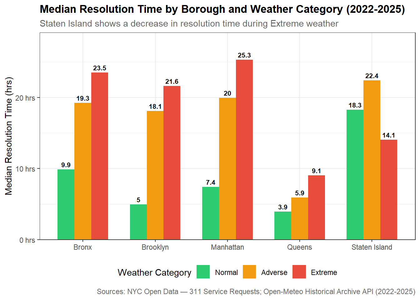
  • Uneven resolution response across boroughs:

    • Queens has the fastest resolution times in all three weather categories.

    • Staten Island is the only borough that experiences faster resolution time than its Normal median but it has the longest median resolution time of all 5 boroughs in every other weather category.

Resolution Time Categories × Weather

Display Code
# Stacked bar chart: proportion of each resolution category by weather category
# Shows whether the distribution of resolution types shifts with weather

# Resolution time categories crossed with weather category
# Adds resolution_category column to the analysis dataset
resolution_cat_weather <- nyc_311_weather_analysis |>
  mutate(
    resolution_category = case_when(
      resolution_hrs <  0.017 ~ "Instant",
      resolution_hrs <  1     ~ "Fast",
      resolution_hrs <  24    ~ "Standard",
      resolution_hrs <  720   ~ "Extended",
      TRUE                    ~ "Long-term"
    ) |> factor(levels = c("Instant", "Fast", "Standard",
                            "Extended", "Long-term"),
                ordered = TRUE)
  ) |>
  group_by(weather_category, resolution_category) |>
  summarise(
    n_requests = n(),
    .groups    = "drop"
  ) |>
  group_by(weather_category) |>
  mutate(pct = round(n_requests / sum(n_requests) * 100, 1)) |>
  ungroup()

# Stacked bar chart: resolution time category distribution by weather category
resolution_cat_weather_chart <- ggplot(resolution_cat_weather,
       aes(x = weather_category, y = pct, 
           fill = resolution_category)) +
  geom_col(width = 0.6) +
  geom_text(
    aes(label = paste0(pct, "%")),
    position = position_stack(vjust = 0.5),
    size     = 3,
    fontface = "bold",
    color    = "white"
  ) +
  scale_fill_manual(
    values = c(
      Instant   = "#2c3e50",
      Fast      = "#2980b9",
      Standard  = "#27ae60",
      Extended  = "#f39c12",
      "Long-term" = "#e74c3c"
    ),
    name = "Resolution Category"
  ) +
  scale_y_continuous(labels = \(x) paste0(x, "%")) +
  labs(
    title    = "Resolution Time Category Distribution by Weather (2022-2025)",
    subtitle = "Extended requests grow during adverse weather while Fast requests decline",
    x        = NULL,
    y        = "% of Requests",
    caption  = "Sources: NYC Open Data — 311 Service Requests; Open-Meteo Historical Archive API (2022-2025)"
  ) +
  theme_bw() +
  theme(
    plot.title      = element_text(face = "bold"),
    plot.subtitle   = element_text(color = "gray40"),
    plot.caption    = element_text(color = "gray40"),
    legend.position = "bottom"
  )

resolution_cat_weather_chart

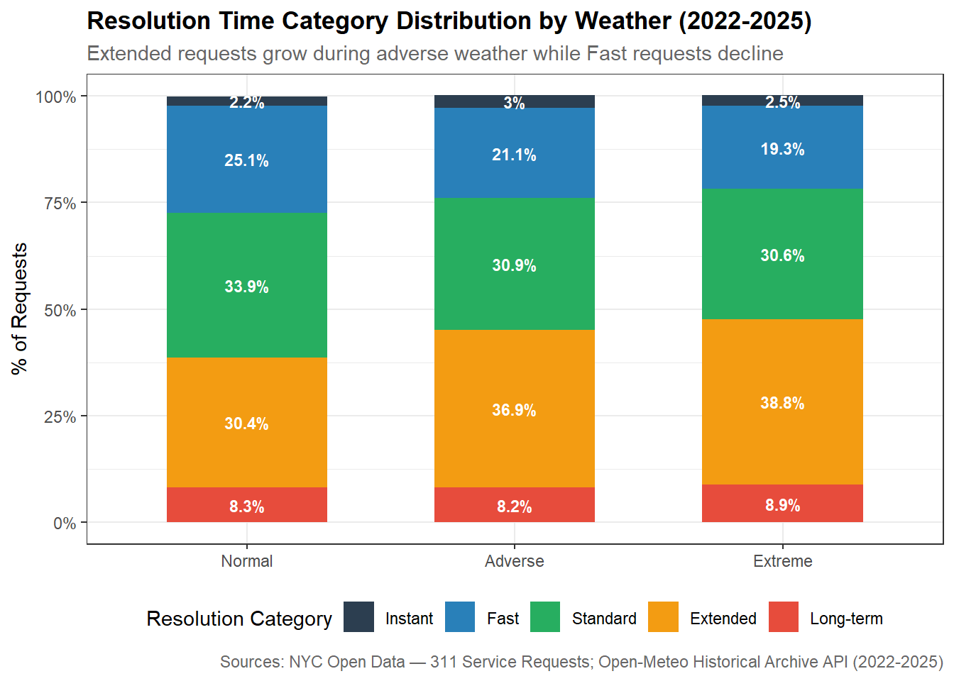
During bad weather, a larger proportion of resolution times shift to Extended (1-30 days). Weather may be pushing requests from the Fast and Standard categories into Extended. The long-term category is largely unaffected by weather conditions but Instant closures increase slightly on Adverse days.

Display Code
# Instant closure rate by agency and weather category
# Focus on high and low volume agencies excluding NYPD initially
# to see if other agencies show interesting patterns
instant_closure_by_agency <- nyc_311_weather_analysis |>
  mutate(
    agency      = str_to_upper(str_trim(agency)),
    is_instant  = resolution_hrs < 0.017
  ) |>
  filter(agency %in% c(high_volume_agencies, low_volume_agencies)) |>
  group_by(agency, weather_category) |>
  summarise(
    n_requests      = n(),
    n_instant       = sum(is_instant),
    pct_instant     = round(mean(is_instant) * 100, 2),
    .groups         = "drop"
  )

# Investigate DEP instant closures on Adverse days
# Check which complaint types are driving the spike
nyc_311_weather_analysis |>
  mutate(
    agency     = str_to_upper(str_trim(agency)),
    is_instant = resolution_hrs < 0.017
  ) |>
  filter(agency == "DEP", is_instant == TRUE) |>
  mutate(complaint_type = str_to_upper(str_trim(complaint_type))) |>
  group_by(weather_category, complaint_type) |>
  summarise(
    n_instant = n(),
    .groups   = "drop"
  ) |>
  group_by(weather_category) |>
  mutate(pct = round(n_instant / sum(n_instant) * 100, 1)) |>
  ungroup() |>
  arrange(weather_category, desc(n_instant)) |>
  group_by(weather_category) |>
  slice_head(n = 5)


# Investigate DSNY instant closures on Extreme days
nyc_311_weather_analysis |>
  mutate(
    agency     = str_to_upper(str_trim(agency)),
    is_instant = resolution_hrs < 0.017
  ) |>
  filter(agency == "DSNY", is_instant == TRUE) |>
  mutate(complaint_type = str_to_upper(str_trim(complaint_type))) |>
  group_by(weather_category, complaint_type) |>
  summarise(
    n_instant = n(),
    .groups   = "drop"
  ) |>
  group_by(weather_category) |>
  mutate(pct = round(n_instant / sum(n_instant) * 100, 1)) |>
  ungroup() |>
  arrange(weather_category, desc(n_instant)) |>
  group_by(weather_category) |>
  slice_head(n = 5)

Regression Model

Display Code
# Linear regression: log(resolution_hrs) ~ weather_category + agency + borough
# Log-transform resolution time to address heavy right skew
# weather_category reference level is Normal — coefficients for Adverse and Extreme show change relative to Normal days
# Agency and borough included as controls to isolate weather effect

# Remove zero resolution times before log transformation
regression_data <- nyc_311_weather_analysis |>
  filter(resolution_hrs > 0) |>
  mutate(
    log_resolution = log(resolution_hrs),
    agency         = str_to_upper(str_trim(agency)),
    # Set Normal as reference level for weather_category
    weather_category = factor(
      as.character(weather_category),
      levels = c("Normal", "Adverse", "Extreme")
    ),
    agency = relevel(factor(agency), ref = "NYPD")
  )

# Fit the model
resolution_model <- lm(
  log_resolution ~ weather_category + agency + borough,
  data = regression_data
)

# Extract tidy coefficients and model fit
model_coefficients <- tidy(resolution_model, conf.int = TRUE)
model_fit          <- glance(resolution_model)

# Display key weather category coefficients
# Back-transform from log scale: exp(coefficient) gives the multiplier
model_coefficients |>
  filter(str_detect(term, "weather_category")) |>
  mutate(
    multiplier  = round(exp(estimate), 3),
    pct_change  = round((exp(estimate) - 1) * 100, 1)
  ) |>
  select(term, estimate, multiplier, pct_change, conf.low, conf.high)

# Shows weather category coefficients back-transformed to multipliers
# and key model fit statistics
Display Code
# Weather coefficients table
regression_table <- model_coefficients |>
  filter(str_detect(term, "weather_category|Intercept")) |>
  mutate(
    term       = recode(term,
      "(Intercept)"             = "Intercept (Normal days)",
      "weather_categoryAdverse" = "Adverse Weather",
      "weather_categoryExtreme" = "Extreme Weather"
    ),
    multiplier = round(exp(estimate), 3),
    pct_change = round((exp(estimate) - 1) * 100, 1)
  ) |>
  select(term, estimate, multiplier, pct_change, conf.low, conf.high) |>
  gt() |>
  tab_header(
    title    = "Regression Results: Weather Effect on Log Resolution Time",
    subtitle = "log(resolution_hrs) Holding Agency and Borough Constant"
  ) |>
  cols_label(
    term       = "Term",
    estimate   = "Coefficient",
    multiplier = "Multiplier",
    pct_change = "% Change",
    conf.low   = "95% CI Lower",
    conf.high  = "95% CI Upper"
  ) |>
  fmt_number(
    columns  = c(estimate, multiplier, conf.low, conf.high),
    decimals = 3
  ) |>
  fmt_number(columns = pct_change, decimals = 1, suffix = "%") |>
  cols_align(align = "left",  columns = term) |>
  cols_align(align = "center", 
             columns = c(estimate, multiplier, pct_change, 
                         conf.low, conf.high)) |>
  tab_style(
    style     = cell_text(weight = "bold"),
    locations = cells_column_labels()
  ) |>
  tab_style(
    style     = cell_fill(color = "#f2f2f2"),
    locations = cells_body(rows = seq(1, 3, by = 2))
  ) |>
  # Add model fit statistics as a footnote
  tab_footnote(
    footnote  = paste0(
      "Adjusted R-squared: ", round(model_fit$adj.r.squared, 3),
      " | Observations: ", scales::comma(model_fit$nobs),
      " | Reference category: Normal weather days"
    ),
    locations = cells_title(groups = "title")
  ) |>
  tab_source_note(
    source_note = "Sources: NYC Open Data — 311 Service Requests; Open-Meteo Historical Archive API (2022-2025)"
  )

regression_table
Regression Results: Weather Effect on Log Resolution Time1
log(resolution_hrs) Holding Agency and Borough Constant
Term Coefficient Multiplier % Change 95% CI Lower 95% CI Upper
Intercept (Normal days) 0.199 1.220 22.0 0.197 0.201
Adverse Weather −0.071 0.932 −6.8 −0.073 −0.068
Extreme Weather −0.249 0.779 −22.1 −0.260 −0.238
1 Adjusted R-squared: 0.649 | Observations: 12,736,820 | Reference category: Normal weather days
Sources: NYC Open Data — 311 Service Requests; Open-Meteo Historical Archive API (2022-2025)

A simple linear regression model analyzes the relationship between resolution time and the predictor variables, weather, agency, and borough. While this can’t establish causation, we can isolate the pure weather effect after accounting for differences caused by agency and borough. Weather categories are the main predictors of interest with Normal as the reference category. The coefficients for Adverse and Extreme tell us how much longer (or shorter) resolution times are compared to Normal days. Resolution times are log transformed to handle the right skew of the data. With 13M rows of data, the p-values will all be essentially zero and not too useful, so I focused on the coefficients of the model and adjusted R2.

Model coefficients are negative for both Adverse (-0.071) and Extreme (-0.249) weather categories, which is counter intuitive given the median analysis earlier indicated longer resolution times during bad weather. The key difference is that regression holds agency and borough constant so once you account for the fact that adverse weather days have a different mix of agencies and boroughs filing complaints, the net weather effect on log resolution time is actually slightly negative.

NoteKey Results
  1. Controlling for agency and borough, Adverse weather is associated with -6.8% change in resolution time and Extreme weather with -22.1% from Normal.

  2. Agency is a dominant predictor. Far more variation in resolution times is explained by which agency handles a request than by weather conditions.

  3. Adjusted R2 of 0.649 means the model explains 64.9% of variation in log resolution times. Agency coefficients do most of the heavy lifting with NYPD (-4.29) and EDC (+3.01) showing enormous differences in baseline resolution times.

Interactive Map

Display Code
if (!requireNamespace("tigris", quietly = TRUE)) {
  install.packages("tigris")
}

library(tigris)

# Download NYC borough boundaries using tigris and cache
# Boroughs are counties in NYC — filter to the 5 NYC counties
options(tigris_use_cache = TRUE)

nyc_boroughs <- counties(state = "NY", cb = TRUE) |>
  filter(NAME %in% c("New York", "Kings", "Queens", "Bronx", "Richmond")) |>
  # Add borough name column to match our 311 data
  mutate(
    borough = case_when(
      NAME == "New York" ~ "Manhattan",
      NAME == "Kings"    ~ "Brooklyn",
      NAME == "Queens"   ~ "Queens",
      NAME == "Bronx"    ~ "Bronx",
      NAME == "Richmond" ~ "Staten Island"
    )
  )


# Aggregate 311 data to borough level for map popups
# One row per borough per weather category
map_data <- nyc_311_weather_analysis |>
  filter(!is.na(borough)) |>
  mutate(complaint_type = str_to_upper(str_trim(complaint_type))) |>
  group_by(borough, weather_category) |>
  summarise(
    n_requests = n(),
    median_hrs = median(resolution_hrs, na.rm = TRUE),
    .groups    = "drop"
  )

# Top 5 complaint types per borough per weather category
top_complaints_by_borough <- nyc_311_weather_analysis |>
  filter(!is.na(borough)) |>
  mutate(complaint_type = str_to_upper(str_trim(complaint_type))) |>
  group_by(borough, weather_category, complaint_type) |>
  summarise(
    n            = n(),
    median_hrs   = median(resolution_hrs, na.rm = TRUE),
    .groups      = "drop"
  ) |>
  group_by(borough, weather_category) |>
  slice_max(n, n = 5) |>
  summarise(
    top_complaints = paste0(
      complaint_type, " (", round(median_hrs, 1), " hrs)",
      collapse = "<br/>"
    ),
    .groups = "drop"
  )

# Join map data with top complaints
map_data <- map_data |>
  left_join(top_complaints_by_borough, by = c("borough", "weather_category"))


# Join map data to borough boundaries
# Need one sf object per weather category for the layer toggles
nyc_boroughs_normal  <- nyc_boroughs |>
  left_join(map_data |> filter(weather_category == "Normal"),
            by = "borough")

nyc_boroughs_adverse <- nyc_boroughs |>
  left_join(map_data |> filter(weather_category == "Adverse"),
            by = "borough")

nyc_boroughs_extreme <- nyc_boroughs |>
  left_join(map_data |> filter(weather_category == "Extreme"),
            by = "borough")

# Colors for weather categories
pal <- colorNumeric(
  palette = c("#2ecc71", "#f39c12", "#e74c3c"),
  domain  = map_data$median_hrs
)

# Popup template function
make_popup <- function(df) {
  paste0(
    "<b>", df$borough, "</b><br/>",
    "<b>Weather Category:</b> ", df$weather_category, "<br/>",
    "<b>Total Requests:</b> ", scales::comma(df$n_requests), "<br/>",
    "<b>Median Resolution Time:</b> ", round(df$median_hrs, 1), " hrs<br/>",
    "<hr/>",
    "<b>Top 5 Complaint Types:</b><br/>",
    df$top_complaints
  )
}

# Build leaflet map with three toggleable layers
nyc_map <- leaflet(
  options = leafletOptions(
    minZoom  = 10,
    maxZoom  = 14,
    zoomSnap = 0.5
  )
) |>
  # Base map tile
  addProviderTiles("CartoDB.Positron") |>
  # Set initial view centered on NYC with zoom level that shows all 5 boroughs
  setView(lng = -73.9857, lat = 40.7484, zoom = 10) |>
  # Constrain map bounds to NYC area to prevent panning to outside NYC
  setMaxBounds(
    lng1 = -74.4,  # Western bound
    lat1 = 40.45,  # Southern bound
    lng2 = -73.65, # Eastern bound
    lat2 = 40.95   # Northern bound
  ) |>
  addPolygons(
    data        = nyc_boroughs_normal,
    group       = "Normal Weather",
    fillColor   = ~pal(median_hrs),
    fillOpacity = 0.7,
    color       = "white",
    weight      = 2,
    popup       = make_popup(nyc_boroughs_normal),
    highlight   = highlightOptions(
      weight       = 3,
      color        = "#333",
      bringToFront = TRUE
    )
  ) |>
  addPolygons(
    data        = nyc_boroughs_adverse,
    group       = "Adverse Weather",
    fillColor   = ~pal(median_hrs),
    fillOpacity = 0.7,
    color       = "white",
    weight      = 2,
    popup       = make_popup(nyc_boroughs_adverse),
    highlight   = highlightOptions(
      weight       = 3,
      color        = "#333",
      bringToFront = TRUE
    )
  ) |>
  addPolygons(
    data        = nyc_boroughs_extreme,
    group       = "Extreme Weather",
    fillColor   = ~pal(median_hrs),
    fillOpacity = 0.7,
    color       = "white",
    weight      = 2,
    popup       = make_popup(nyc_boroughs_extreme),
    highlight   = highlightOptions(
      weight       = 3,
      color        = "#333",
      bringToFront = TRUE
    )
  ) |>
  addLayersControl(
    baseGroups = c("Normal Weather", "Adverse Weather", "Extreme Weather"),
    options    = layersControlOptions(collapsed = FALSE)
  ) |>
  addLegend(
    pal      = pal,
    values   = map_data$median_hrs,
    title    = "Median Resolution<br/>Time (hrs)",
    position = "bottomright"
  ) |>
  hideGroup("Adverse Weather") |>
  hideGroup("Extreme Weather")

nyc_map
Conclusion

For most of the bad weather types we examined (save for extreme heat), resolution times were longer but weather may not be the sole reason behind this increase. Citywide median resolution time increased 2.5x more than Normal on Adverse days and 3.4x on Extreme days. However, this aggregate number masks dramatically different agency-level responses. The regression model confirms that controlling for agency and borough, the pure weather effect is actually modest, which suggests that what appears to be a weather effect is partially a composition effect driven by which agencies handle weather-driven complaint surges.

Weather may slightly impact resolution times but not equally across agencies and the type of work an agency does may determine how sensitive it is to adverse conditions. A two-tier service response emerges for field agencies and administrative agencies. Field based agencies are more affected by weather and slow down significantly during adverse weather. This may be because demand surges faster than capacity or bad weather poses a blocker (for example, health inspectors at DOHMH can’t get to restaurants because of heavy snow). DPR and DOT are two field agency standouts since they handle a lot of storm related requests (like fallen trees) and consistently resolve issues faster during adverse weather. The work of administrative/enforcement agencies such as NYPD are less affected by adverse weather conditions.

Regression analysis confirmed that agency type is the strongest predictor of weather sensitivity. Our overarching question asks whether factors driving resolution times suggest segmented prioritization of issues and this weather analysis provided three pieces of evidence against this:

  • Several agencies appear to resolve requests faster during adverse weather but this is driven by bulk instant closure behavior rather than genuine efficiency. DEP and DSNY were top offenders in this regard. This may be evidence of reactive triage to manage complaint volume rather than active prioritization.

  • While some weather-specific complaints were serviced quicker, the most weather-critical complaints experienced bottlenecks and slower resolution. Complaint types most directly driven by adverse weather and residents need resolved quickly during adverse conditions show longer resolution times during bad weather (ex: Heat/Hot Water 30% slower on Adverse days). The system didn’t proactively prioritize the most weather-critical complaints especially when demand may outpace capacity.

  • Resolution times during bad weather are unevenly distributed across boroughs adding a geographic dimension to the question of prioritization

Regression analysis supports a conclusion that it is not weather that determines the resolution times but the agency response and the composition of different issues that occur during bad weather events. Coupled with weather-related complaint bottlenecks, we can see that these findings suggest that 311’s service system responds to adverse weather through reactive triage and capacity constraints rather than deliberate prioritization of the most weather-critical issues.

Claude was used to help write the code in this project and brainstorm final deliverable ideas, but all non-code text was generated without the use of any Generative AI tools.


This work ©2025 by Evelyn Rodriguez was initially prepared as a Course Project for STA 9750 at Baruch College. More details about this course can be found at the course site and instructions for this assignment can be found at Final Project